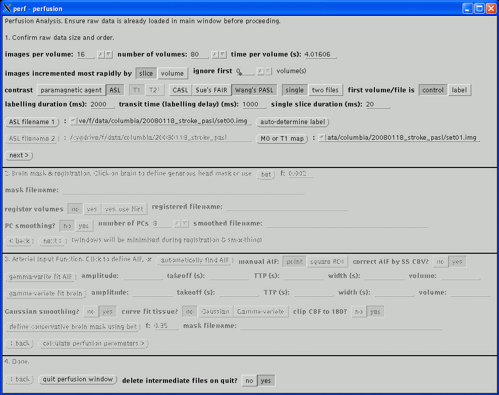
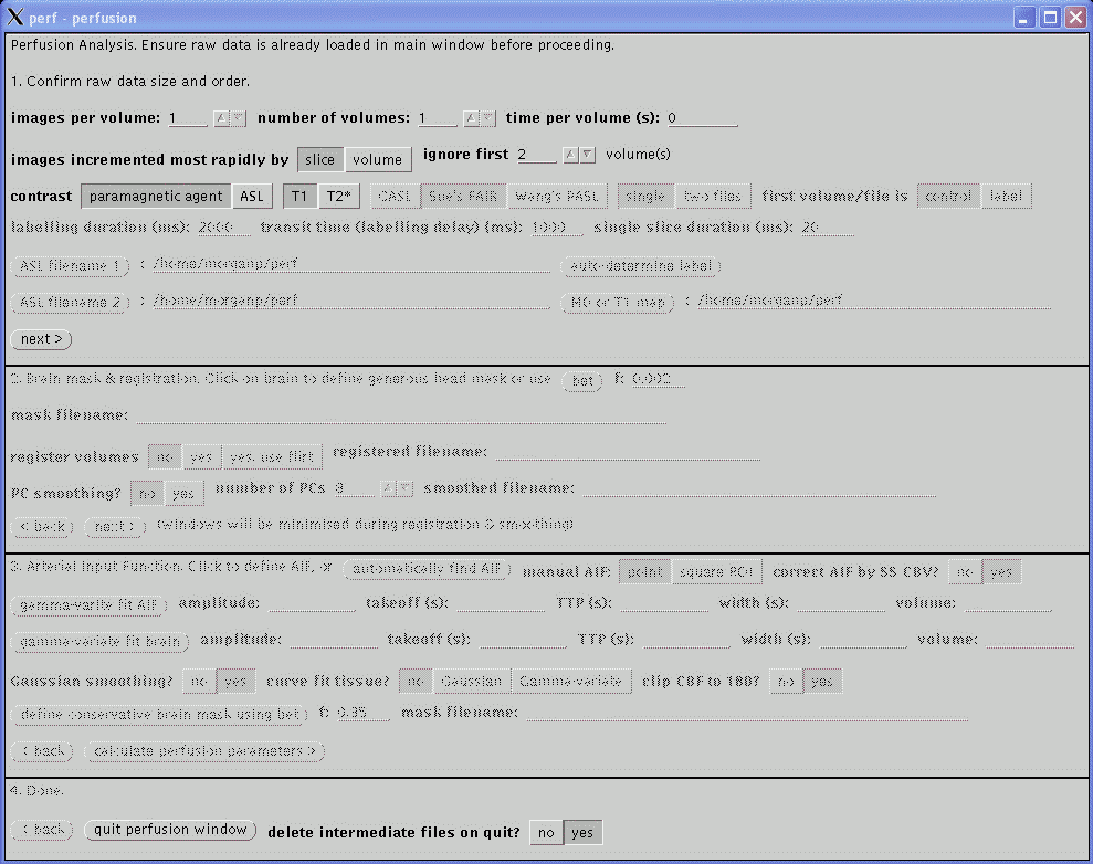
This section confirms the actual acquisition parameters to use for the perfusion analysis and take precedent over the values read from the image file header.
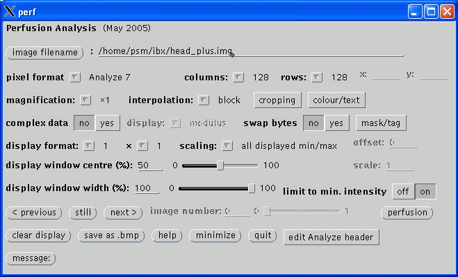
The images per volume and number of volumes are usually read correctly. If unsure, return to the main window and scroll through the images (using the previous and next buttons) to asssertain the correct values.
The time per volume value is often not present in the image header and should be checked carefully. If the value is left at zero, the gamma-varite fit of the Arterial Input Function will fail below and just yield a horizontal green line. If the value is non-zero but incorrect, the perfusion parameters will not be quantified. The value in Analyze headers will usually be wrong; if a PAR/REC file has been loaded, the value should be correct so long as extra dummy volumes have not been prescribed. Its value is typically in the range 1 to 4 seconds.
The images incremented most rapidly by slice or volume option indicates the image order in the file. The order may be assertained by returning to the main window and scrolling through the images, as described above (note, at this stage, images will always scroll in the order in which they are stored in the file regardless of the setting of this option). slice indicates that each increment of an image in the file displays another slice, i.e., the images are stored volume by volume. volume indicates that each increment of an image displays a different time point for the same slice, i.e., the images are stored as time series. This option will usually be slice for PAR/REC files and may be either for Analyze files depending on how they were converted. Analyze files created using MRIcro from DICOM or PAR/REC files will be incremented by slice as will Analyze files converted from PAR/REC using ptoa. Currently, Philips DICOM files converted using dtoa will be incremented by volume. Also see swap34.
The number of volume to be ignored are the beginning of the time series is specified by the ignore first .. volumes setting. Initial volumes are not considered in the analysis as the signal takes a few repetitions to reach a steady state value. However, do not set this value too high as a few steady state dynamic volumes are required in the analysis prior to the arrival of the bolus in order to determine the baseline signal. If 'dummy' volumes are acquired and discarded by the scanner this value may be set to zero.
The contrast mechanism being exploited to measure the perfusion parameters may be selected. Analysis of exogenous paramagnetic contrast agent is supported, exploiting either T1 or T2* weighting. If T2* is selected, only relative perfusion parameters will be calculated. Continuous Arterial Spin Labelling analysis currently only works on data acquired using Philips MR scanners and uses a similar post-processing algorithm to the Philips Pride CASL tool. Currently, quantification of CASL assumes that the images were acquired at 3 T data.
If CASL has been selected, the following options become available and values must be entered.
The labelled and non-labelled Analyze files must be selected. The only valid file format is Analyze. Analyze files may have been converted from either DICOM (using dtoa) or PAR/REC (using ptoa). Data converted using MRIcro should also work but this has not been tested. If MRIcro is used for conversion of Philips data, ensure that the Calibrate scaling [Philips data only] option is selected under Etc / Options. If this option is not present, download a more recent version of MRIcro.
If the Analyze files were converted using dtoa then the labelled and non-labelled file may be automatically discriminated by clicking auto-determine label.
The labelling duration and transist time values must be entered, in milliseconds. These values are not recorded in either the DICOM or PAR files and must be noted from the scanner user interface. On Philips scanners, these values are on the Dyn/ang page.
Click next> to advance to the next stage. All the slices in the last volume of the dynamic acquisition should be loaded and displayed correctly. If not, click <back from the second section and correct the parameters in this section to ensure correct image ordering.
Now the type and form of the data have been defined, this section deals with motion correction and smoothing of the images prior to calculation of the perfusion parameters. When analysising new data it might be useful to set all options in this section to No and proceed to stage three to obtain a quick overview of the perfusion results. Then return to this section to select the appropriate options which will hopefully result in a better perfusion calculation.
Defining a generous mask around the head will speed up the registration and visually improve the results. At any time while the second section is active clicking in the brain in any of the displayed images will result in the generation of a binary mask which will be displayed. The mask is saved to a file, the filename of which is displayed as mask filename. If the displayed mask is inappropriate or a mask is not required, manually deleted this filename. Alternatively, the filename of a mask file created using other software may be entered; however, clicking on the images subsequently will result in a new mask being generated by the perfusion software. To display the actual images again after the mask has been defined, click on the still button in the main window.
The mask generation algorithm used by the perfusion software is not very sophisticated and often results in a poor mask. In these cases, manually delete the mask filename. An option to use BET to define a mask will be added in the future.
Motion correction is performed by setting register volumes to yes. Registration is performed using the dynamic_3d_reg program which must be in the PATH and should be in Paul Morgan's bin sub-directory. This uses the mask, if defined above, and may take some time to perform depending on the amount of images and the speed of the computer (10 to 60 minutes is not uncommon). An option to use FLIRT will be added in the future. Registration will be started when next> is clicked at the bottom of section two and once started may only be interrupted by killing the process from UNIX. During registration, the graphical windows will be minimised. Progress will be displayed in the command window in which perf was started. This option is intended to be used on the raw MR images - if the images have already been realigned and resampled to a standard space, resulting in a large number of slices per volume, this option should not be selected as it will take a very long time to perform.
Following motion correction (if selected), principle component PC smoothing of the images may be selected (option not available for ASL). This usually helps reduce noise in the data without loosing spatial resolution but may be susceptible to image artefacts and gross patient movement. The number of PCs determines how many components are used in the final data, where the first PC should be the background, the second PC the arterial phase of the data, the third PC the veneous phase, and so on. Values between 4 and 10 are reasonable with lower values resulting in less noise but may compromise the dynamic detail of the data. PC smoothing is much quicker to perform that motion correction but may still take a few minutes to perform. As with motion correction, the graphical windows will be minimised during the calculation.
The smoothed filename value will be filled in automatically by the calculations in this section and will be the data used by the third section, below. If motion correction and PC smoothing have already been performed on the data, both these options may be set to No before proceeding to the next stage to prevent the calculations being performed again.
Click next> to advance to the next stage, at which point the calculations for any of the options selected in this section will be performed and the windows may be minimised.
The T1 perfusion technique requires an arterial input function (AIF) to enable quantification. The T2* technique does not require an AIF but one should be defined anyway as a check the quality of the bolus of contrast agent. CASL does not require a AIF; continue to the next stage of the analysis by clicking next>.
The AIF should be in an artery, not a vein, and should show the largest change in amplitude as the bolus passes. The automatically find AIF button tries to find the best AIF in the data and displays a green cross over the pixel used. The time course of that pixel is plotted as a graph in a new window. When using the automatic function, check that the green cross does not erroneously appear in a vein, usually the sagittal sinus. If this occurs, you will have to define the AIF manually (see below).
To define the AIF manually, move the cursor (now in the shape of a cross) over the images and click on an appropriate arterial point to display the time course. A carotid artery in one of the lower slices usually provides the best AIF. The manual AIF may be chosen as the point under the cross, or by setting the manual AIF option to square ROI, the 'best' AIF within a 16x16 square cursor is found and selected. A green cross will represent the position of the new AIF, although the images may need to be refreshed (e.g., by clicking the still button) to display the most recently defined AIF location.
An example of an automatically defined AIF is shown below. The location of the AIF time course is indicated by the green cross over the subject's left internal carotid artery in image 0, volume 15.
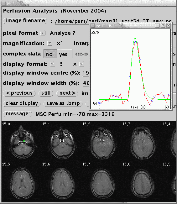
Once a suitable AIF has been identified, it is necessary to fit a gamma-variate curve to the data. This eliminates effects of recirculation of the bolus of contrast agent and provides the characteristics of the AIF used in the calculation of perfusion parameters. In the perfusion window, click gamma-variate fit AIF. The fit is displayed on the AIF curve as a green line. Some parameters from the fit are displayed (amplitude, takeoff, width, volume). Check that the green curve is a reasonable fit to the data (in red). If it is not, there is not much interactive adjustment that can be performed, other than to pick another AIF. If just a horizontal line is displayed, check that the time per volume in section one, above, is reasonable, in units of seconds, and non-zero. If the AIF in the raw data appears hard up against the left hand side of the graph, reduce the ignore first .. volume(s) value in section one.
After fitting the AIF, click gamma-variate fit brain to fit to the agregate brain curve. This defined start and end points for the CBV calculation. The program does not check that the gamma-variate fits of the AIF and brain have been performed, or belong to the current data set, but if this is not the case, erroneous perfusion parameters will be calculated.
The calculated maps of perfusion parameters may be smoothed. 3x3 smoothing is selected by setting Gaussian smoothing to Yes. The curve fit tissue? option should always be set to No.
Click calculate perfusion parameters> to calculate the maps of perfusion parameters.
The perfusion maps have bee saved to disk, named after the original filename with '_perf', '_cbv', and '_ttp' added for maps of CBF, CBV, and TTP. They can be viewed using this 'perf' program or 'ibx'. For ASL acquisitions, no TTP image is saved and the CBV image contains the percentage signal change between labelled and non-labelled images.
Click <back to return to the previous section to edit parameters. Continue to click the relevant <back buttons to return to the first section before closing the perfusion window by clicking quit perfusion window at the bottom of the window.
The delete intermediate files on quit option will delete all extra files created during post-processing, such as the PC smoothed images, if set to Yes. Only the original data and final perfusion parameter maps will remain. Leave this set to Yes for routine processing.