Dilation of VOIs

Using MRIcron to investigate perfusion and diffusion values in regions around lesions at MUSC

This page briefly describes the practical steps required to analyze MRI diffusion and perfusion data, using FSL, Java Image, and MRIcron to produce diffusion and perfusion values from rings of dilated VOIs around a brain lesion, specifically for the brain tumor patient study in Radiology & Radiological Sciences at MUSC.

1. Retrieve Patients from PACS using OsiriX

Use the dual-monitor Mac. (Leo Bonilha will know its location if it gets moved, or if the username and password are required.)
Start OsiriX
Click Query.
In the new window, select the Patient ID tab. Enter the patient's Medical Record Number (MRN).
In the list of the patient's appointments, select the appropriate scan date and ensure the modality for that appointment includes MR.
Click Retrieve. This takes less than one minute per patient.
Repeat searching and retrieving all patients. Several Retrieves can be run in parallel.

2. Export DICOM from OsiriX

Back in the OsiriX main window, highlight all patients for export (hold down the Apple key while selecting multiple patients).
Click Export.
Browse to the required destination folder on the Mac's System HD (e.g., /morgan ).
Create a new folder (using the button lower left) with a unique name that does not contain any spaces (e.g., tumor_todays_date ).
Click Choose. Wait for the DICOM export to finish.

3. Transfer DICOM to the CAIR hornet server

Open a Terminal window on the Mac. Type the following, replacing username with your hornet username, and tumor_todays_date with the name of the folder into which you exported the DICOM images, above.
```
cd /morgan
scp -r tumor_todays_date username@147.120.124.11:/data/studies_large/morganp/tumor/dicom
```
Once successfully transferred, the tumor_todays_date folder that you created on the Max can be deleted. The patients can also be deleted from OsiriX to save more disk space - they can always be re-retrieved from PACS.

4. Connect to the CAIR hornet server using VNC

Information on installing on new local PCs may be viewed on the MUSC CAIR Sharepoint site. New users should first contact John Dornisch.
Use VNC to connect to the CAIR hornet server (IP address 147.120.124.11 ).
Convert the newly transferred DICOM images to Analyze format by typing the following in a terminal window -
```
cd /data/studies_large/morganp/tumor
dtoa -ana -delses -over -datefirst -fdt dicom/tumor_todays_date
```
This creates new patient subdirectories in /data/studies_large/morganp/tumor named by the MR scan date and patient name.
It also produces diffusion MD and FA maps from the appropriate images automatically, although this can take some time to process after conversion by dtoa has completed; typically look for the creation of the MD and FA image files in the patients' folder after about 30 minutes per new patient. However, you can start processing the perfusion data in parallel.

5. Process perfusion data using JIM

5.1 Indentify input images

Change into the patient subdirectory on hornet. Identify the file containing the perfusion raw data. If the DICOM files were converted using dcm2nii then the filename should indicate the name of the acquisition protocol used. If dtoa was used for conversion, type showana *.hdr | grep desc to list the acquisition protocol used for each image file.
The raw perfusion data file will contain a name similar to ep2d_perf if acquired on a Siemens MR scanner, or PERF/PRESTO if acquired on a Philips MR scanner.
However, more than one image file may contain this identifier, as this label may also be attached to images produced by the scanner's on-line perfusion processing package. If this is the case, each image file containing the perfusion label should be inspected. The raw perfusion image file will contain multiple dynamic volume measurements, whereas the on-line perfusion processed results will normally only contain one volume. To determine the number of dynamic volumes, either type showana image_filename and examine the line starting 'images per volume', or use graphical software such as MRIcro to display the number of volumes.
Once the perfusion raw data image file has been indentified, display related information required by the perfusion processing software by typing showana image_filename In particular, note the TE from the 'description' line, the 'number of volumes', and the 'volume duration'.

5.2 Initial settings for JIM

Start the Java Image software by typing jim &
The first time you run Jim, I suggest modifying some of the preferences as follows. Select Toolkits / Preferences. Under the Misc tab, set
- I work most often with: Analyze images
- I like my NIFTI images in: One file .nii
- I like my NIFTI images: Compressed
- Also select a more relevant startup directory.
Click Save Settings on this tab, then select the Interoperability tab.
- Tick the Create new Analyze 7.5 images only with non-flipped orientations box
then click Save Settings and Done.

5.3 Perfusion Analysis

From the main menu, select Toolkits / Brain Perfusion. In the new Perfusion Analysis window, accept the default parameter values except as discussed below.
Input configuration: Select Single input image. Click on the folder icon then browse and select the perfusion raw data file that you identified. above. File browsing with JIM in general can take a bit of getting used to, in particular, it appears best to always browse for a file graphically (rather than typing its name in manually), and when double clicking to select a sub-directory, it's more successfully to double click on the folder icon to the left of the folder name rather than on the folder name itself.
Input configuration: The Number of time points in image is the number of volumes displayed by showana image_filename above.
Input configuration: The Time between images can usually be determined from the volume duration displayed by showana image_filename above. It should be in the range of about 0.5 - 4 seconds. Depending on the source DICOM file, the volume duration displayed by showana may be correct, or it may be the time for the entire acquisition in which case you will need to divide it by the number of volumes first. Also remember to convert from ms to s.
Input configuration: Leave the Number of steady state images as 1 as for the protocols at MUSC these will alreayd have been discarded as 'dummies' on the scanner. Select Register images to perform motion correction. Optionally select Apply smoothing filter (but once you have decided whether to use it or not, be consistent for all subjects). Rather than use Brain Finder, you can define a brain mask by applying FSL's BET to the first volume of the raw perfusion data after the JIM perfusion analysis has finished.
Threshold: Typically a value of 80 should be okay.
Quantification parameters: For the Scan TE enter the TE value from the description line displayed by showana above. Leave the other parameters in this section at their default values.
Arterial Input Function: The delay between start of the scan and the first arrival of the contrast agent in the brain can vary between patients depending on their heart rate, age, and the relative time that the injection was actually initiated. The parameters listed here appear to work for the current perfusion protocol at MUSC, and one would hope that the MRI techs always time the perfusion scans consistently. However, this may not always be the case, not least due to new MR scanners being installed, software upgrades, or the decision to modify the perfusion protocol. During the perfusion analysis, below, the AIF graph is displayed on the screen containing dots to indicate at what point the analysis started to look for contrast. If this is right at the start of the rising curve, you should probably reduce the Scan number at contrast arrival by 2 and re-run the analysis. Likewise, if the dot on the graph is well before the curve starts to rise, the initial pre-contrast baseline interval may be too short resulting in a poor estimate of the baseline value which will affect the perfusion calculation, and so the Scan number at contrast arrival should be increased and the analysis re-run.

Example of varying Scan Number At Contrast Arrival parameter

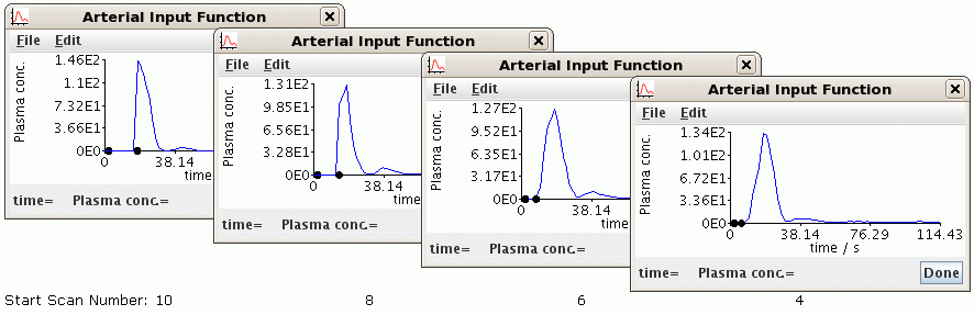
Try a value of 8 for Scan number at contrast arrival and a value of one less than the number of dynamic volumes, for the Analysis end scan number.
When you become more familiar using JIM, there is also an option to plot the timecourse of individual pixels, or ROIs, using the Dynamic Analysis - Roaming Intensities tool.
AIF selection: Automatic.
Output folder: Select this graphically, to be the same as the folder containing the input raw perfusion image files. Click Load to accept the folder selection.
Output base name: Type this in manually. I suggest appending "_perf" to the input filename, so if the input filename is set09.hdr the use an Output base name of set09_perf
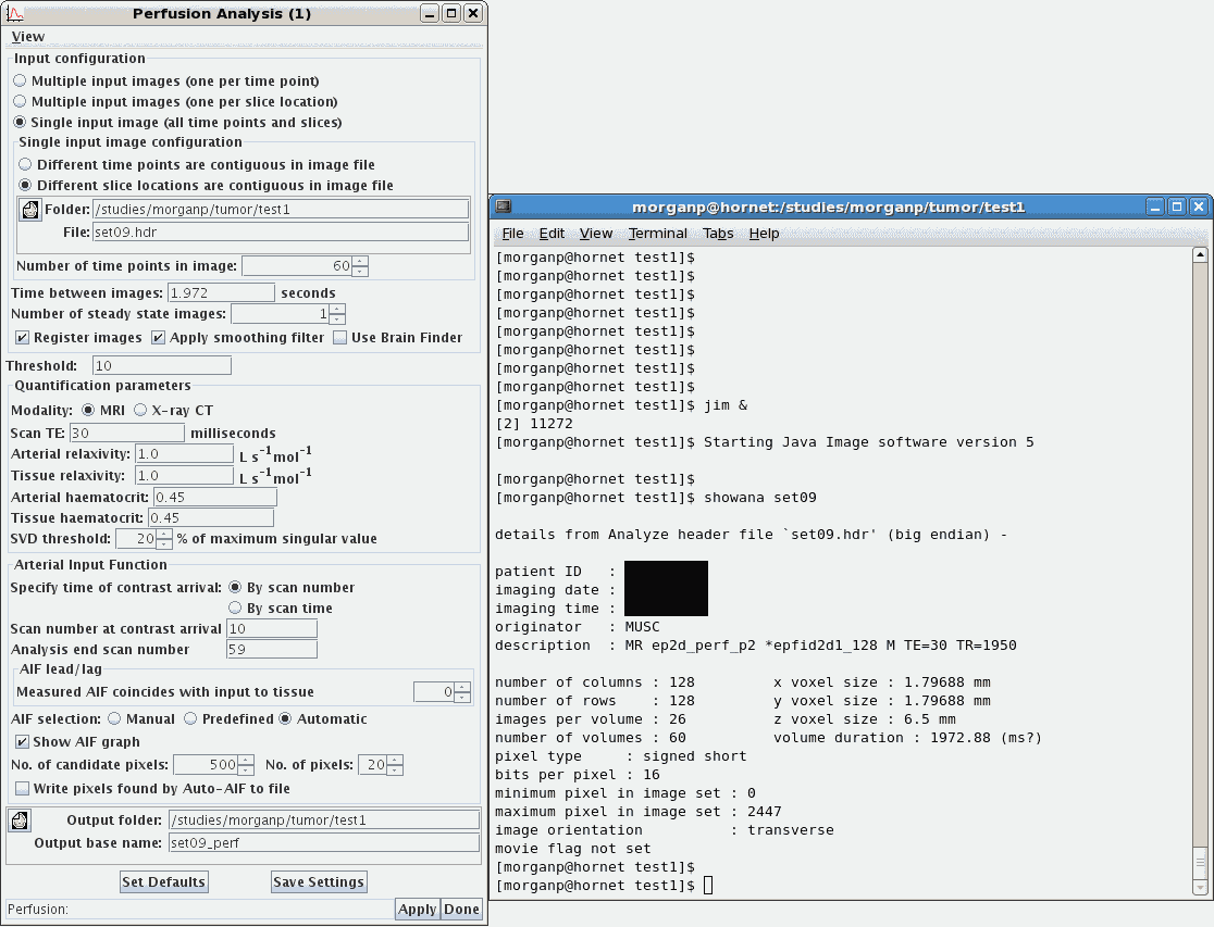
Click Apply to start the analysis.

5.4 Check results and generate brain mask

Load one of the perfusion images (e.g., the CBV map) into an image viewing program to check they look reasonable. Do not use JIM for this, but use MRIcron, MRIcro, fslview, or ibx, all of which are available on the hornet server. Check that the images appear reasonable and are the right way up. If the images are upside down, check your preference settings as described in section 5.2, above, and then re-run the perfusion analysis.
Create a brain mask. For a later stage of analysis, below, this mask needs to be in MRIcron VOI format. Create this mask as follows.
Start MRIcron by typing mricron &
Select File / Open and load in the raw perfusion scans. As this is a dynamic multi-volume acquisition, you will be prompted for which volume number to load. Select the first volume.
Select Draw / Advanced / Brain Extraction. Reduce the default 0.5 factor to 0.2 and click Go.
If the resulting images look reasonable, then close the Brain Extraction window and select Draw / Advanced / Brain Mask. This will prompt to save the brain mask in VOI format. Choose a filename with the same base name as the perfusion acquisition, e.g., if the perfusion raw data were in a file named set09 then name the VOI file something like set09_brain_mask

6. Draw VOI using MRIcron

Usually the Volume Of Interest will be drawn on the FLAIR image. Indentify which file contains the FLAIR using a similar process as in section 5.1, above, i.e., by typing showana *.hdr | grep desc
FLAIR scans acquired on a Siemens scanner may contain the name FLAIR or tir2d in the decription field. Acquisitions on a Philips scanner are usually labeled FLAIR.
Start MRIcron by typing mricron &
Check the options in the Help / Preferences page. Ensure that the Show drawing menus and tools option is selected. Also note the Reorient images when loading option. This should be unselected before loading the FLAIR images for drawing the VOIs. However, selecting it and reloading the FLAIR scans may make visual assessment of the lesion and final VOI easier.
Select File / Open to load the FLAIR image file.
Scroll through the slices and identify the lesion. Draw round the lesion, as instructed by the neuroradiologist, slice by slice.
Draw by first clicking on the Autoclose pen button then click and hold while drawing with the mouse. After completing the region on each slice, fill the region by either right clicking in it, or by using the Fill tool button.
Repeat for all slices. Save by selecting Draw / Save VOI...
(To view the VOI in interpolated 3D, select the Reorient images when loading option, see above, then reload the FLAIR scans, then select Draw / Open to reload the VOI file. Scroll through the orthogonal slices by clicking the crosshair.)

7. Dilate VOI using MRIcron

Start MRIcron and load the processed perfusion map (e.g., CBV or CBF).
Load the VOI drawn on the FLAIR, above, by selecting Draw / Open VOI. Especially if using a combination of NIFTI images, check that a left-right flip has not occurred, and that the VOI overlays as expected. Note, this stage is just a visual check; you will re-select these images again during the dilation process below.
Select Draw / Advanced / Dilate VOIs
The next prompt asks for the number of boundaries for the dilations around the surface of the VOI. So, for example, to obtain four adjacent dilated bands around the core VOI, enter 5 edges.
Enter the distance of the edges of the dilations away from the VOI surface. Entering 0, 5, 10, 15, 20 will result in four dilated bands around the core VOI, where band 1 ranges from 0-4 mm, band 2 from 5-9 mm, band 3 from 10-14 mm, and band 4 from 15-19 mm. Dilations occur in 3D.
You then have the option to mask the dilated VOIs with an additional mask. This is useful to prevent the dilations extending outside the brain, or to constrain the dilations to a particular hemisphere, or to just white matter. In the case, select Yes and choose the brain mask created above in section 5.4. To select the VOI file containing the brain mask created above, first change the File of type: pull down menu to Volume of interest (*.voi).
In the next Select VOI browser window, reselect the VOI file that outlines the core lesion.
The next Select PERF image browser window requires the filename of the post-processed perfusion image to analyse (CBV, CBF, etc.).
The dilated VOIs are then generated, and saved. The next Select VOI browser window is prompting to repeat the analysis with a different core lesion VOI. Click Cancel, and a Descriptive Statistics window will open containing the results from each dilated band around the core lesion. It may be easier to save these data (File / Save) and view the results in another editor or spreadsheet. the values in this file are the values from whichever perfusion parametr file was selected above, e.g., CBV, CBF, etc.

8. Non-perfusion data

While the instructions on this page relate to analysis of perfusion images, the same technique can be applied to other parameter maps, such as diffusion maps of ADC (or MD). The perfusion maps will need to be generated, but then the dialation stage is the same as in section 7, above, except that instead of selecting perfusion parameter map of CBV or CBF, instead select the diffusion ADC image.

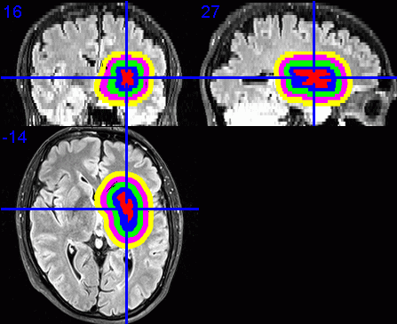
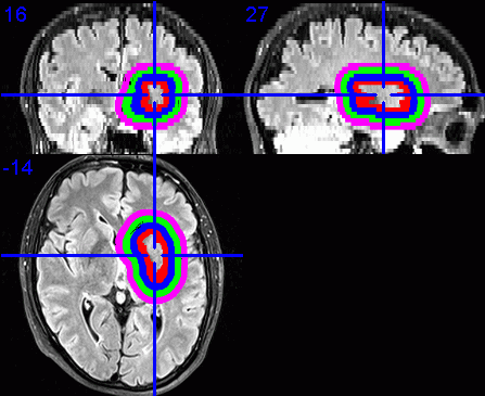
9. Visualisation of dilated VOIs

To visualise the dilated VOIs using MRIcron, I suggest first enabling the Reorient images when loading setting, as described in the fourth point in section 6 above.
Load the required base images, e.g., the FLAIR images.
Select Overlay / Add. Change the Files of type: to VOIs and choose the core lesion VOI file.
Repeat the step above, expect each time select the VOI file for the next dilated band. The VOI filenames start with a 1, 2, 3, ... depending on the level of dilation, followed by the name of the core VOI. Each VOI should be displayed in a different colour.
Click on the centre of the lesion to obtain the required view of the VOIs in the three orthogonal planes.
Select File / Save as Bitmap to save this view as an image that could be inserted into a document or presentation.